
Gritty Graphs - Elections (1/3)
It’s election season, and we are going to have a look at a lot of interesting activities at the voter level across different states. While politics is very interesting to study, it may be useful for us to take a step back and see the broader trends in the country. In this episode of gritty graphs, we will explore some of these trends. A useful resource for this is the India votes database that’s available to us free of charge from Ashoka university’s site : Data Set
This is a pretty big data set and just doing surface work would not do justice to it so we will continue to drill deeper into this. You can also try and see if you get any insights, maybe we would be able to collaborate.
Let’s load the data
data<- read.csv("TCPD GE All States Mar 15.csv")Now, once you download the data, it’s pretty straightforward for us to clean it.
library(tidyverse)
data.select.1<- data %>%
  select(
    Year, State_Name, Constituency_Name, Valid_Votes, Electors
  ) %>%
  unique() %>%
  group_by(State_Name, Year) %>%
  summarise(
    Valid_Votes =sum(Valid_Votes),
    Electors = sum(Electors)
  ) %>%
  mutate(
    voter.turnout = Valid_Votes/Electors
  )
Now, we will need to start looking not at the state level but at a macro level. Let’s define regions and see what happens.
# Define the states
states <- c("Andaman_&_Nicobar_Islands", "Andhra_Pradesh", "Arunachal_Pradesh", "Assam",
            "Bihar", "Chandigarh", "Chhattisgarh", "Dadra_&_Nagar_Haveli", "Daman_&_Diu",
            "Delhi", "Goa", "Gujarat", "Haryana", "Himachal_Pradesh", "Jammu_&_Kashmir",
            "Jharkhand", "Karnataka", "Kerala", "Lakshadweep", "Madhya_Pradesh",
            "Maharashtra", "Manipur", "Meghalaya", "Mizoram", "Nagaland",
            "Odisha", "Puducherry", "Punjab", "Rajasthan", "Sikkim",
            "Tamil_Nadu", "Telangana", "Tripura", "Uttar_Pradesh", "Uttarakhand",
            "West_Bengal", "Dadra & Nagar Haveli And Daman & Diu", "Goa,_Daman_&_Diu",
            "Mysore", "Madras")

# Create a vector to categorize states into regions
region <- rep("", length(states))

# Assign states to their respective regions
region[states %in% c("Andhra_Pradesh", "Karnataka", "Kerala", "Tamil_Nadu", "Telangana", "Puducherry", "Lakshadweep", "Mysore", "Madras")] <- "South Indian"
region[states %in% c("Odisha", "West_Bengal", "Assam", "Arunachal_Pradesh", "Manipur", "Meghalaya", "Mizoram", "Nagaland", "Tripura", "Andaman_&_Nicobar_Islands", "Sikkim")] <- "East Indian"
region[states %in% c("Madhya_Pradesh", "Chhattisgarh", "Jharkhand")] <- "Central Indian"
region[states %in% c("Haryana", "Himachal_Pradesh", "Jammu_&_Kashmir", "Punjab", "Uttarakhand", "Uttar_Pradesh", "Delhi", "Chandigarh", "Bihar")] <- "North Indian"
region[states %in% c("Gujarat", "Maharashtra", "Rajasthan", "Goa", "Daman_&_Diu", "Dadra_&_Nagar_Haveli", "Dadra & Nagar Haveli And Daman & Diu", "Goa,_Daman_&_Diu")] <- "West Indian"

# Combine the data into a data frame
state_regions <- data.frame(State_Name = states, Region = region)

data.select.1<- left_join(data.select.1, state_regions)
Now, let’s simply plot it.
# Convert voter turnout to percentage
data.select.2$voter.turnout <- data.select.2$voter.turnout * 100

# Create the line plot
ggplot(data.select.2, aes(x = Year, y = voter.turnout, group = Region, color = Region)) +
  geom_line() +
  labs(title = "Voter Turnout by Region and Year",
       x = "Year",
       y = "Voter Turnout (%)") +
  theme_minimal()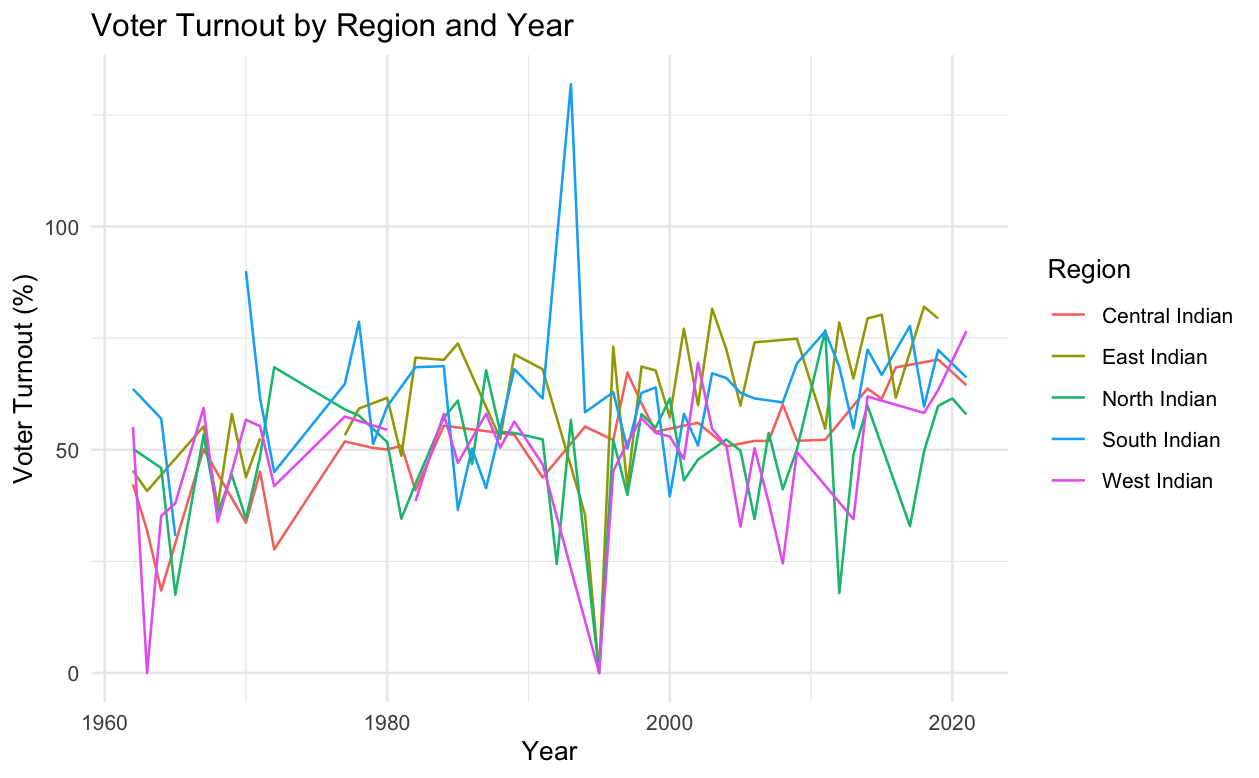
This is our output. Let’s try and understand it..
There appears to be some sort of spike in 1997 or so in the south. It says there is over 100% voting. How can that be? However, the opposite seems to be the case with West India.
To be honest, this looks really cluttered. And we are not able to decipher the insights we want. Would it not be nice to see the individual lines side by side? This is where the fine art of faceting comes in.
Faceting is a powerful tool for data visualization, particularly when dealing with multifaceted and layered data. It allows us to split one plot into multiple plots based on a categorical variable, each showcasing a slice of the data. In essence, it creates a matrix of panels defined by rows and columns, with each panel showing a subset of the data. This technique is extremely helpful when comparing groups or trends across different categories and can reveal patterns or anomalies that might be obscured in a combined single plot. By isolating each category, we maintain a consistent scale and context while allowing each subplot to stand on its own for comparative analysis. Faceting thus helps to declutter complex data visualizations, making them more readable and insightful.
Let me show you.
# Create the line plot with vertical x-axis labels
ggplot(data.select.2, aes(x = Year, y = voter.turnout, group = Region, color = Region)) +
  geom_line() +
  labs(title = "Voter Turnout by Region and Year",
       x = "Year",
       y = "Voter Turnout (%)") +
  theme_minimal() +
  theme(axis.text.x = element_text(angle = 90, hjust = 1, vjust = 0.5)) +
  facet_grid(~Region)
This gives us:
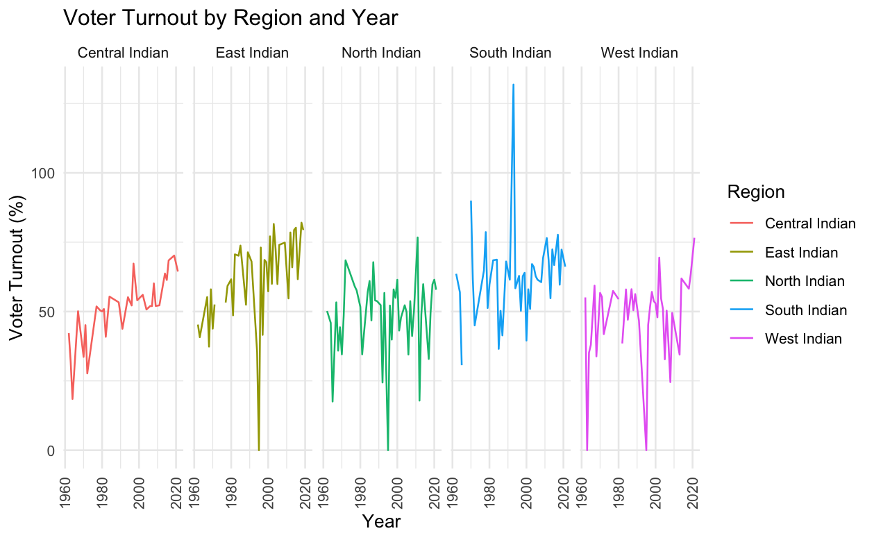
This seems like time got compressed. A little bit of extra tinkering can help us over come this:
# Create the line plot with vertical x-axis labels and facet wrap into 5 rows
ggplot(data.select.2, aes(x = Year, y = voter.turnout, group = Region, color = Region)) +
  geom_line() +
  labs(title = "Voter Turnout by Region and Year",
       x = "Year",
       y = "Voter Turnout (%)") +
  theme_minimal() +
  theme(axis.text.x = element_text(angle = 90, hjust = 1, vjust = 0.5)) +
  facet_wrap(~ Region, nrow = 5)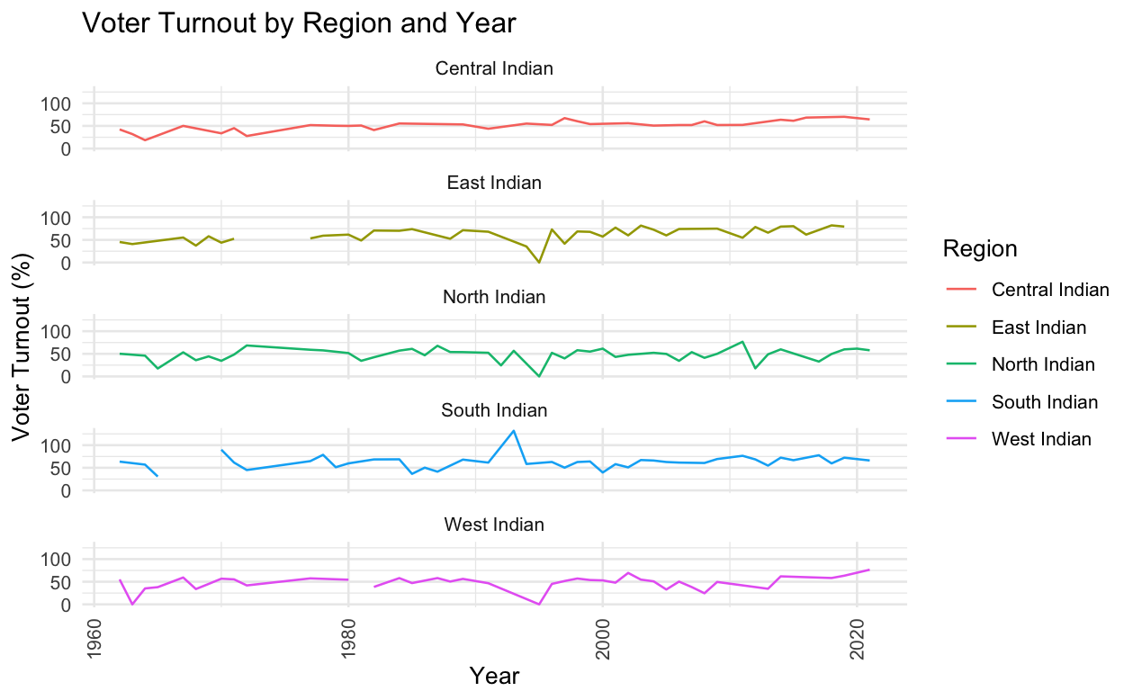
Essentially. It’s true. There appear to be a few cases in which extreme voter turnouts have happened. We’ll have to investigate this further. But then, you get the idea.
In conclusion, faceting has transformed our approach to understanding voter turnout across various regions in India. The technique has disentangled the complex web of data, enabling us to discern regional patterns and outliers with greater clarity. With this improved visualization, we uncovered intriguing trends, such as the unusually high turnout in the south during 1997 and the contrasting patterns in the west. These findings prompt a deeper dive into the data, guiding us toward targeted inquiries and meaningful interpretations. Faceting isn't just a feature of our graphing toolset—it's a window into the nuanced narrative of voter behavior, inviting both experts and novices alike to engage with the data in a dialogue of discovery. As we peel back layers of data, each facet serves as a chapter in the unfolding story of India's electoral dynamics.
By using faceting, we are able to showcase and observe every region (think of this as a category) to the best possible ability - this is something that can be quite invaluable when we have to understand competing but equally important categories.
In the next few issues, we’ll make this our theme. Let’s dissect and discern the truth from the data that we have with us, thanks to Ashoka University.
You can find the link to the code on our GitHub Repository.